
TL;DR
A client recently approached me with an interesting challenge. They wanted another layer of verification in their manufacturing quality control process. Technicians were occasionally missing defects, and time pressures meant inspection reports weren’t always completed.
This struck me as a good opportunity to explore local AI. The client was a smaller business looking for something tailored to their needs rather than an off-the-shelf solution. More importantly, the potential business value wasn’t necessarily cost reduction or revenue growth, but risk reduction. Could AI act as a second set of eyes and help technicians catch something they might otherwise miss?
There was also a practical requirement: inspections sometimes happen in locations without reliable connectivity. I therefore wanted to start by proving that image analysis could run locally, rather than depend on a cloud AI service.
This is the story of what I built, the approaches that didn’t work, and why I eventually used a pre-trained computer vision model rather than training a neural network myself. Longer term, I can see potential for Microsoft Foundry to help with inspection context and reporting, but that’s for a later stage.
[Download it on GitHub here].
Architecture and approach
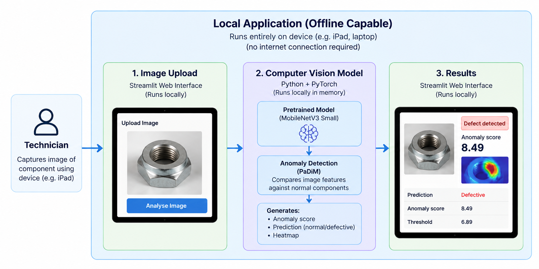
The architecture
The longer-term idea is an application that technicians could access on a device such as an iPad. They’d capture an image of a component and receive an indication of anything unusual, together with a heatmap highlighting areas worth checking.
The intention isn’t to replace the technician’s judgement or carry out the initial inspection. That’s their area of expertise. The AI would provide an additional verification step.
For this POC, I used Python, PyTorch and Streamlit, with the computer vision model running on my MacBook Air. Streamlit provided a simple browser interface. Once the model weights and dependencies were available locally, image analysis could run without an internet connection. That demonstrates local inference on a laptop, not a model running natively on an iPad. Deploying it to technicians would require further work, either to run inference on their devices or on a nearby edge computer.
Getting started
I used my existing MacBook Air with an M1 chip and 8GB of RAM. Not exactly a dedicated AI workstation, but I wanted to see what was possible without immediately provisioning a cloud GPU!
Initially, I considered Ollama and one of Microsoft’s Phi models, given that I spend most of my time working with Microsoft technologies. But this wasn’t a language problem. I needed to analyse images and identify potential defects, so a specialised computer vision model was a better fit. I eventually used MobileNetV3 Small, a lightweight pretrained model available through Torchvision.
I created a project directory and virtual environment:
mkdir industrial-defect-ai
cd industrial-defect-ai
python3 -m venv .venv
source .venv/bin/activate
Then installed the libraries for the experiments and application:
pip install torch torchvision
pip install transformers datasets accelerate
pip install scikit-learn pandas matplotlib pillow
pip install streamlit
The Hugging Face packages were part of my initial exploration; I didn’t ultimately need them for the final detector.
PyTorch supports Apple’s Metal Performance Shaders (MPS), which lets supported operations use the integrated GPU. I checked that it was available with:
import torch
device = torch.device(
“mps” if torch.backends.mps.is_available() else “cpu”
)
print(device)
This returned mps. With only 8GB of unified memory, I still had to be sensible about model size, batch sizes and image resolution, but it was enough to experiment locally.
Finding a dataset
One lesson I learnt quickly was that getting an AI model running is often easier than finding relevant, usable data!
The client had previous inspection images, but they needed reviewing and organising. For an initial POC, I decided to leave that work for later and use MVTec AD, a dataset designed for industrial anomaly detection research.
I chose its metal-nut category because the components were reasonably similar to some of the client’s inspection images. It contains 220 normal training images and 115 separate test images, covering normal components and defects such as scratches, bends, colour changes and flipped nuts. It also includes masks showing where defects appear, useful for evaluating heatmaps.
I kept the dataset’s original train/good, test and ground_truth structure under data/mvtec/metal_nut/. Crucially, the separate test set meant I could check how well an approach worked on unseen images.
Choosing an approach
My initial assumption was that I’d need to train a neural network to recognise defective components. I was also keen to get some hands-on experience with model training, so I tried several approaches. Working on the M1 meant I could explore these without cloud GPU costs, although the hardware naturally limited how ambitious I could be.
What I hadn’t appreciated was that I could use a pretrained neural network to extract visual features, then use a separate anomaly detection method to establish what normal components look like. That still requires normal images to build a baseline, but it doesn’t require retraining the neural network’s weights.
Of course, I only worked that out after going down something of a cul-de-sac!
First attempt: image classification
I started with MobileNetV3 Small, pretrained on ImageNet. I adapted its classification layer to distinguish normal and defective images, then trained the modified network using labelled examples.
from torchvision.models import mobilenet_v3_small, MobileNet_V3_Small_Weights
model = mobilenet_v3_small(
weights=MobileNet_V3_Small_Weights.DEFAULT
)
The results weren’t convincing: the model identified some defects but also flagged too many normal components. Worse, I discovered I’d accidentally included official test images in the training and validation process. That’s data leakage: the model may have seen images it was later evaluated on, making those results unreliable.
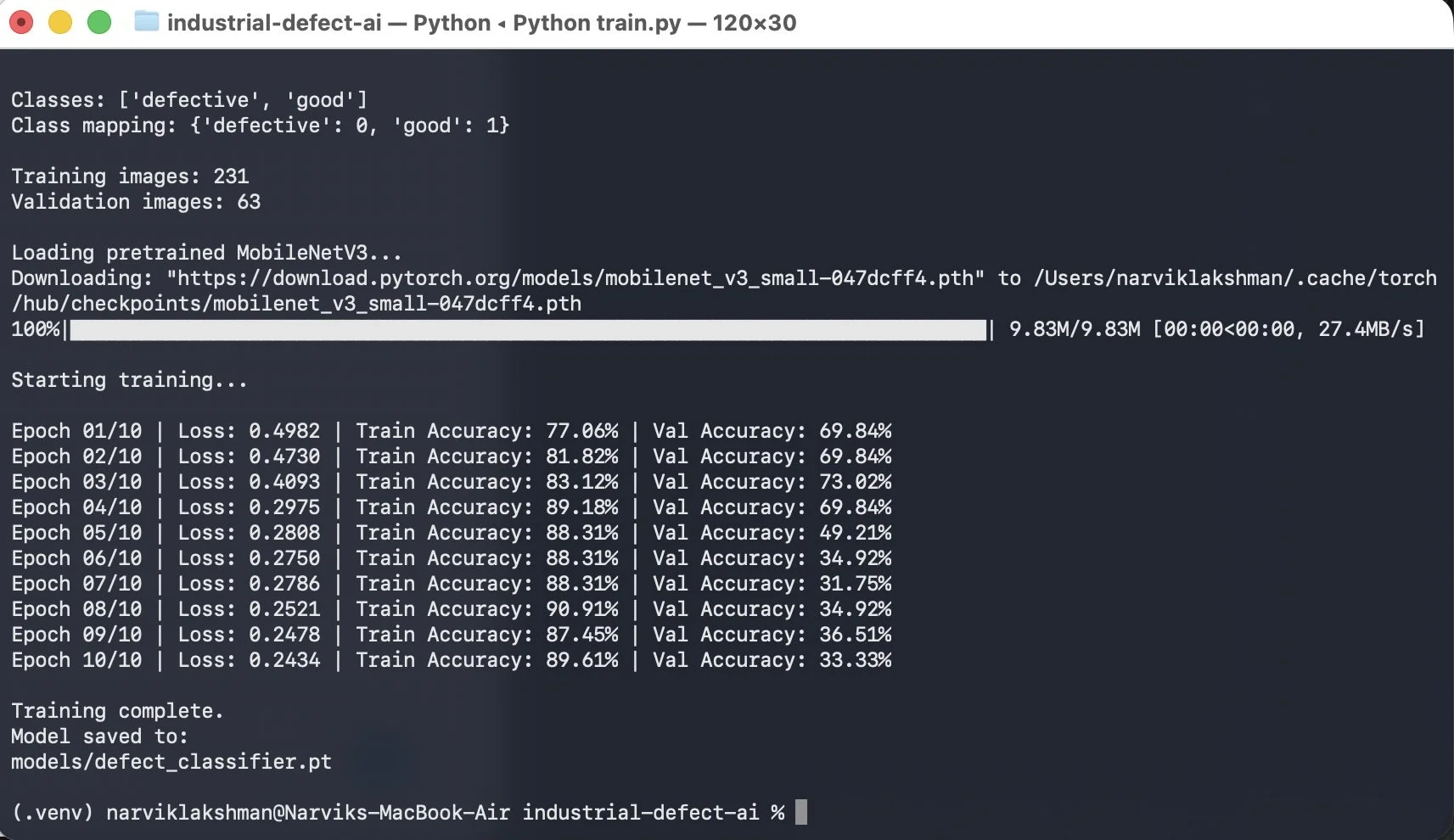
Initial MobileNetV3 training results. Training accuracy reached almost 90%, while validation accuracy fell to 33%, showing that the model wasn’t generalising well.
It also made me question classification as the right approach. In manufacturing, you can’t necessarily anticipate every possible defect. Would we need to collect and label new examples every time something unexpected appeared?
Anomaly detection seemed more suitable: establish what normal looks like and flag deviations, including potentially unfamiliar defects.
Second attempt: an autoencoder
An autoencoder is a neural network trained to reconstruct images. The theory is that, after training on normal components, it should reconstruct those reasonably well but struggle with defective ones. The reconstruction difference becomes an anomaly score.
Here I was training a neural network, updating its weights to reduce reconstruction error. The core of that process looked like this (the complete implementation is in the repository):
reconstructed = model(images)
loss = criterion(reconstructed, images)
loss.backward()
optimizer.step()
Unfortunately, my implementation achieved only around 19% accuracy, detecting very few defects. Autoencoders can sometimes reconstruct defective areas surprisingly well while introducing errors elsewhere, so reconstruction error doesn’t always separate normal and defective images reliably.
I could have spent longer tuning it, but decided to explore another approach.
Third attempt: pretrained features
I returned to MobileNetV3 Small, but stopped trying to train it as a classifier. Instead, I used its existing ability to extract visual patterns such as shapes, edges and textures.
model.eval()
for parameter in model.parameters():
parameter.requires_grad = False
with torch.no_grad():
features = model.features(images)
The neural network’s weights stayed unchanged. I extracted features from normal images and used nearest-neighbour comparisons to see how different new images were.
Comparing whole-image features achieved around 58% accuracy. The problem was that a small scratch could get lost when most of the component still looked normal.
So I tried patch-based features, comparing smaller image regions. Accuracy improved to around 77%. Combining features from different layers and increasing image resolution eventually produced around 89% in one high-resolution patch experiment.
That was the turning point: examining individual regions was much more effective for small defects, and I was doing it without retraining MobileNetV3.
Moving to PaDiM
I then explored PaDiM (Patch Distribution Modelling). Instead of comparing a new image with individual normal examples, PaDiM describes the statistical distribution of normal features at different locations in an image.
I built a PaDiM-style detector using features from two layers of MobileNetV3 Small. For each location, I calculated the average and covariance of features extracted from normal components. This provided a statistical baseline.
This was my own lightweight implementation using MobileNetV3 Small, rather than an exact reproduction of the original PaDiM architecture.
For new images, I used Mahalanobis distance to measure how unusual their features were relative to that baseline, accounting for how features normally vary together. The result was an anomaly score for each region, which I could turn into a heatmap.
I used the average of the highest-scoring 5% of patches as the overall image score. Of the 220 normal training images, 176 built the baseline and 44 calibrated the threshold for flagging a component as defective. I then tested the detector on the separate official test set.
The results
| Metric | Result |
| — -| — -:|
| Overall accuracy | 88% |
| Defect recall | 86% |
| Defect precision | 99% |
| F1 score | 0.92 |
| Pixel-level AUROC | 0.9574 |
Of 93 defective components, the detector identified 80 and missed 13. It also correctly classified 21 of 22 normal components, incorrectly flagging just one.
Because the test dataset contains considerably more defective images than normal ones, overall accuracy doesn’t tell the whole story. Defect recall and the number of false positives were therefore particularly important when assessing the results.
For an initial POC, I was pretty happy with that. I’d achieved approximately 88% accuracy locally, using a lightweight pretrained neural network without retraining its weights or calling a cloud AI service. The pixel-level AUROC was encouraging too, suggesting the heatmaps were generally distinguishing defective regions from normal ones.
The earlier high-resolution patch experiment had slightly higher image-level accuracy at around 89%, but the PaDiM-style approach offered a useful statistical scoring method and heatmaps for the application.
Although the earlier high-resolution patch experiment achieved slightly higher accuracy, I decided to continue with the PaDiM-style approach because I wanted to explore its statistical anomaly scoring method and use the resulting anomaly maps in the application.
It’s worth remembering the original objective: an additional check for a technician, not an automated decision replacing their expertise. The results suggested the approach had potential. The next step would be testing it on actual client images, including variations in lighting, angles and backgrounds, and seeing how far performance could be improved.
As I’d used the MVTec dataset throughout my experiments, I’d also want to validate the final approach against a completely independent set of images. The results demonstrate feasibility rather than independently validated production accuracy
Building the application
Until this point, I’d been running Python scripts. I wanted something a technician could actually interact with, so I built a simple interface in Streamlit.
The application accepts an image, preprocesses it, extracts MobileNetV3 features, calculates anomaly scores, applies the threshold and displays the result with a heatmap. Streamlit’s uploader made the interface straightforward:
uploaded_file = st.file_uploader(
“Upload a component image”,
type=[“jpg”, “jpeg”, “png”]
)
I launched it locally using:
streamlit run app.py
Naturally, the first test uncovered another problem! The application flagged a normal component as defective, despite the evaluation results looking reasonable.
It turned out that the application and evaluation scripts were calculating Mahalanobis distance differently: one used the squared distance and the other its square root. The scores and threshold were therefore on different scales.
After fixing that, a normal component scored 5.857 against a threshold of 6.891, while a defective component scored 8.490 and was correctly flagged.
It was a useful reminder that a working model isn’t the same as a working application. Consistent preprocessing and scoring matter just as much when you integrate everything.
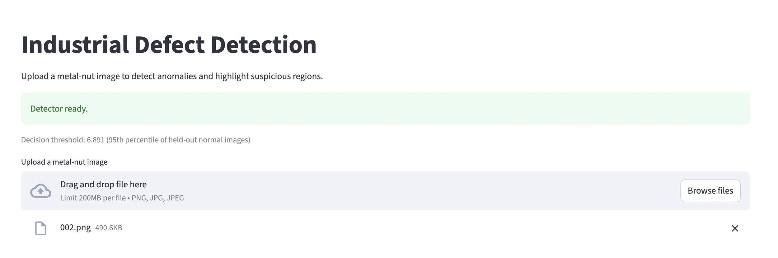
The Streamlit interface
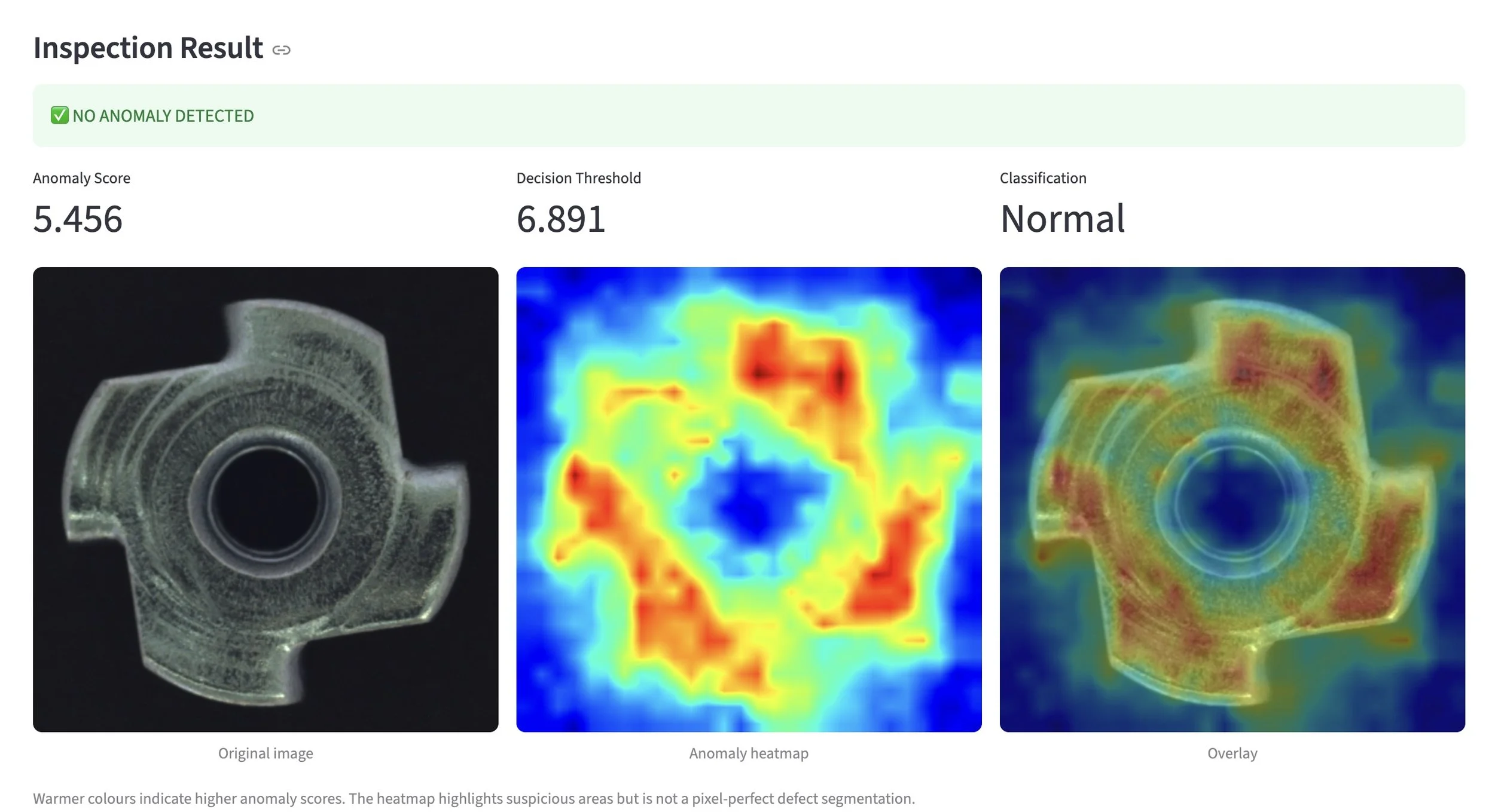
Inspection result for a normal metal nut
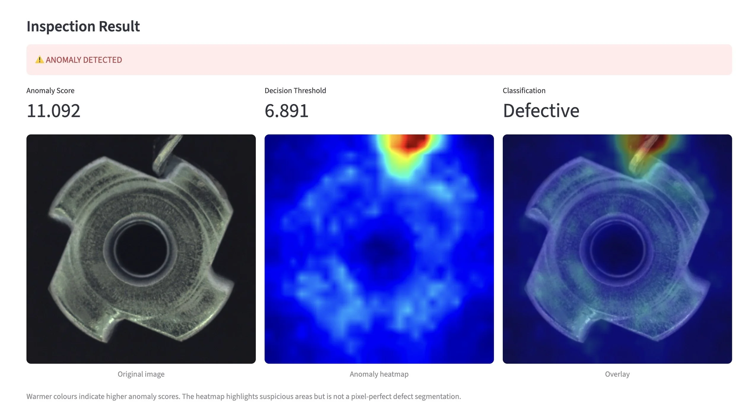
Inspection result for a bent metal nut (see how it heatmaps the anomaly)
What I learned and what’s next
The POC isn’t a finished field solution. I still need to test actual client images and work out how disconnected inspections would operate on technicians’ devices, including local storage and synchronisation. But it demonstrated that local computer vision could provide a practical starting point.
My biggest takeaway was that I didn’t need to train a neural network myself to get useful results. I did need normal images to fit the statistical anomaly detector, but MobileNetV3’s pretrained weights could stay exactly as they were.
I also learnt a fair bit about dataset quality, data leakage and the importance of keeping evaluation and application code consistent. And, perhaps most importantly, this reinforced that not every AI problem needs an LLM or a cloud service.
Longer term, I’d like to explore a hybrid approach using Microsoft Foundry. The local detector can highlight unusual regions, but it doesn’t know the manufacturer’s quality standards, previous inspection history or what needs to go into a report. A cloud-based model or agent could potentially combine those sources with technician notes and generate a draft report for review when connectivity is available.
The idea would be local inspection first, cloud assistance when available, without making the core inspection dependent on a network connection. I haven’t built that part yet, but it could address the other half of the client’s challenge: helping technicians complete inspection reports.
Ultimately, I wanted to explore how AI could solve a real business problem rather than build something simply for the sake of using AI. The experiment gave me a working local POC, a better understanding of what works and a few lessons from what didn’t!
As you can probably tell I’m a total amateur at this so I’d be interested to hear any feedback and whether others have been exploring similar local or hybrid AI use cases and what you’ve do.